| |

Artificial Neural NetworksAt earlier times, the conventional computers incorporated algorithmic approach that is the computer used to follow a set of instructions to solve a problem unless those specific steps need that the computer need to follow are known the computer cannot solve a problem. So, obviously, a person is needed in order to solve the problems or someone who can provide instructions to the computer so as to how to solve that particular problem. It actually restricted the problem-solving capacity of conventional computers to problems that we already understand and know how to solve. But what about those problems whose answers are not clear, so that is where our traditional approach face failure and so Neural Networks came into existence. Neural Networks processes information in a similar way the human brain does, and these networks actually learn from examples, you cannot program them to perform a specific task. They will learn only from past experiences as well as examples, which is why you don't need to provide all the information regarding any specific task. So, that was the main reason why neural networks came into existence. Artificial Neural Network is biologically inspired by the neural network, which constitutes after the human brain. Neural networks are modeled in accordance with the human brain so as to imitate their functionality. The human brain can be defined as a neural network that is made up of several neurons, so is the Artificial Neural Network is made of numerous perceptron. 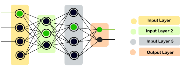
A neural network comprises of three main layers, which are as follows;
Motivation behind Neural NetworkBasically, the neural network is based on the neurons, which are nothing but the brain cells. A biological neuron receives input from other sources, combines them in some way, followed by performing a nonlinear operation on the result, and the output is the final result. 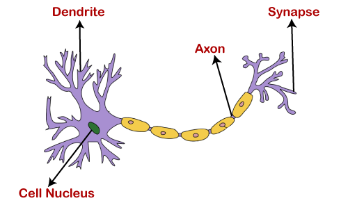
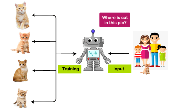
The dendrites will act as a receiver that receives signals from other neurons, which are then passed on to the cell body. The cell body will perform some operations that can be a summation, multiplication, etc. After the operations are performed on the set of input, then they are transferred to the next neuron via axion, which is the transmitter of the signal for the neuron. What are Artificial Neural Networks?Artificial Neural Networks are the computing system that is designed to simulate the way the human brain analyzes and processes the information. Artificial Neural Networks have self-learning capabilities that enable it to produce a better result as more data become available. So, if the network is trained on more data, it will be more accurate because these neural networks learn from the examples. The neural network can be configured for specific applications like data classification, pattern recognition, etc. With the help of the neural network, we can actually see that a lot of technology has been evolved from translating webpages to other languages to having a virtual assistant to order groceries online. All of these things are possible because of neural networks. So, an artificial neural network is nothing but a network of various artificial neurons. Importance of Neural Network:
Working of Artificial Neural NetworksInstead of directly getting into the working of Artificial Neural Networks, lets breakdown and try to understand Neural Network's basic unit, which is called a Perceptron. So, a perceptron can be defined as a neural network with a single layer that classifies the linear data. It further constitutes four major components, which are as follows;
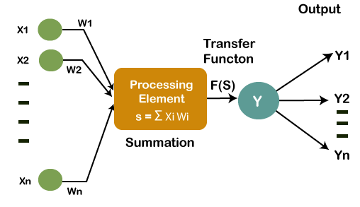
The main logic behind the concept of Perceptron is as follows: The inputs (x) are fed into the input layer, which undergoes multiplication with the allotted weights (w) followed by experiencing addition in order to form weighted sums. Then these inputs weighted sums with their corresponding weights are executed on the pertinent activation function. Weights and BiasAs and when the input variable is fed into the network, a random value is given as a weight of that particular input, such that each individual weight represents the importance of that input in order to make correct predictions of the result. However, bias helps in the adjustment of the curve of activation function so as to accomplish a precise output. Summation FunctionAfter the weights are assigned to the input, it then computes the product of each input and weights. Then the weighted sum is calculated by the summation function in which all of the products are added. Activation FunctionThe main objective of the activation function is to perform a mapping of a weighted sum upon the output. The transformation function comprises of activation functions such as tanh, ReLU, sigmoid, etc. The activation function is categorized into two main parts:
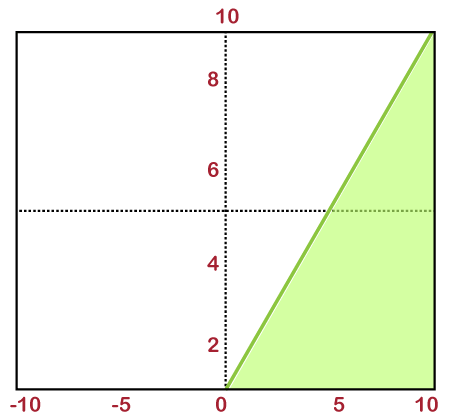
Linear Activation FunctionIn the linear activation function, the output of functions is not restricted in between any range. Its range is specified from -infinity to infinity. For each individual neuron, the inputs get multiplied with the weight of each respective neuron, which in turn leads to the creation of output signal proportional to the input. If all the input layers are linear in nature, then the final activation of the last layer will actually be the linear function of the initial layer's input. 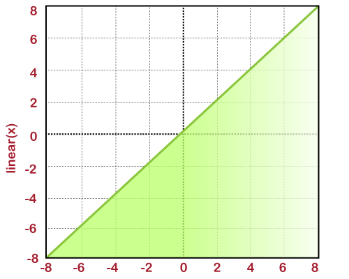
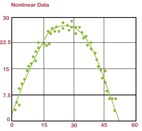
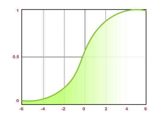
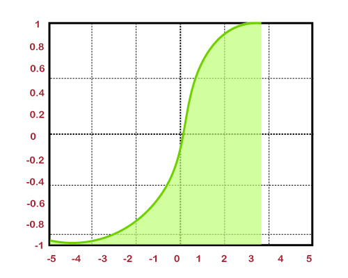
Non- linear functionThese are one of the most widely used activation function. It helps the model in generalizing and adapting any sort of data in order to perform correct differentiation among the output. It solves the following problems faced by linear activation functions:
The non-linear activation function is further divided into the following parts:
Gradient Descent AlgorithmGradient descent is an optimization algorithm that is utilized to minimize the cost function used in various machine learning algorithms so as to update the parameters of the learning model. In linear regression, these parameters are coefficients, whereas, in the neural network, they are weights. Procedure: It all starts with the coefficient's initial value or function's coefficient that may be either 0.0 or any small arbitrary value.
coefficient = 0.0
For estimating the cost of the coefficients, they are plugged into the function that helps in evaluating.
cost = f(coefficient)
or, cost = evaluate(f(coefficient)) Next, the derivate will be calculated, which is one of the concepts of calculus that relates to the function's slope at any given instance. In order to know the direction in which the values of the coefficient will move, we need to calculate the slope so as to accomplish a low cost in the next iteration.
delta = derivative(cost)
Now that we have found the downhill direction, it will further help in updating the values of coefficients. Next, we will need to specify alpha, which is a learning rate parameter, as it handles the amount of amendments made by coefficients on each update.
coefficient = coefficient - (alpha * delta)
Until the cost of the coefficient reaches 0.0 or somewhat close enough to it, the whole process will reiterate again and again. It can be concluded that gradient descent is a very simple as well as straightforward concept. It just requires you to know about the gradient of the cost function or simply the function that you are willing to optimize. Batch Gradient DescentFor every repetition of gradient descent, the main aim of batch gradient descent is to processes all of the training examples. In case we have a large number of training examples, then batch gradient descent tends out to be one of the most expensive and less preferable too. Algorithm for Batch Gradient Descent Let m be the number of training examples and n be the number of features. Now assume that hƟ represents the hypothesis for linear regression and ∑ computes the sum of all training examples from i=1 to m. Then the cost of function will be computed by: Jtrain (Ɵ) = (1/2m) ∑ (hƟ(x(i)) - (y(i))2 Repeat { Ɵj = Ɵj - (learning rate/m) * ∑ (hƟ(x(i)) - y(i)) xj(i) For every j = 0...n } Here x(i) indicates the jth feature of the ith training example. In case if m is very large, then derivative will fail to converge at a global minimum. Stochastic Gradient DescentAt a single repetition, the stochastic gradient descent processes only one training example, which means it necessitates for all the parameters to update after the one single training example is processed per single iteration. It tends to be much faster than that of the batch gradient descent, but when we have a huge number of training examples, then also it processes a single example due to which system may undergo a large no of repetitions. To evenly train the parameters provided by each type of data, properly shuffle the dataset. Algorithm for Stochastic Gradient Descent Suppose that (x(i), y(i)) be the training example Cost (Ɵ, (x(i), y(i))) = (1/2) ∑ (hƟ(x(i)) - (y(i))2 Jtrain (Ɵ) = (1/m) ∑ Cost (Ɵ, (x(i), y(i))) Repeat { For i=1 to m{ Ɵj = Ɵj - (learning rate) * ∑ (hƟ(x(i)) - y(i)) xj(i) For every j=0...n } } Convergence trends in different variants of Gradient DescentThe Batch Gradient Descent algorithm follows a straight-line path towards the minimum. The algorithm converges towards the global minimum, in case the cost function is convex, else towards the local minimum, if the cost function is not convex. Here the learning rate is typically constant. However, in the case of Stochastic Gradient Descent, the algorithm fluctuates all over the global minimum rather than converging. The learning rate is changed slowly so that it can converge. Since it processes only one example in one iteration, it tends out to be noisy. BackpropagationThe backpropagation consists of an input layer of neurons, an output layer, and at least one hidden layer. The neurons perform a weighted sum upon the input layer, which is then used by the activation function as an input, especially by the sigmoid activation function. It also makes use of supervised learning to teach the network. It constantly updates the weights of the network until the desired output is met by the network. It includes the following factors that are responsible for the training and performance of the network:
Working of BackpropagationConsider the diagram given below. 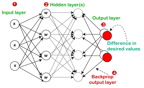
Need of Backpropagation
Building an ANNBefore starting with building an ANN model, we will require a dataset on which our model is going to work. The dataset is the collection of data for a particular problem, which is in the form of a CSV file. CSV stands for Comma-separated values that save the data in the tabular format. We are using a fictional dataset of banks. The bank dataset contains data of its 10,000 customers with their details. This whole thing is undergone because the bank is seeing some unusual churn rates, which is nothing but the customers are leaving at an unusual high rate, and they want to know the reason behind it so that they can assess and address that particular problem. Here we are going to solve this business problem using artificial neural networks. The problem that we are going to deal with is a classification problem. We have several independent variables like Credit Score, Balance, and Number of Products on the basis of which we are going to predict which customers are leaving the bank. Basically, we are going to do a classification problem, and artificial neural networks can do a terrific job at making such kind of predictions. So, we will start with installing the Keras library, TensorFlow library, as well as the Theano library on Anaconda Prompt, and for that, you need to open it as administrator followed by running the commands one after other as given below. Since it is already installed, the output will be as given below. 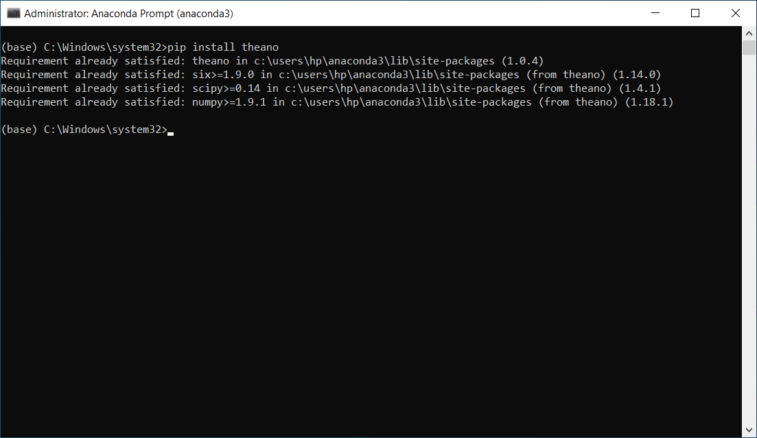
From the image given below, it can be seen that the TensorFlow library is successfully installed. 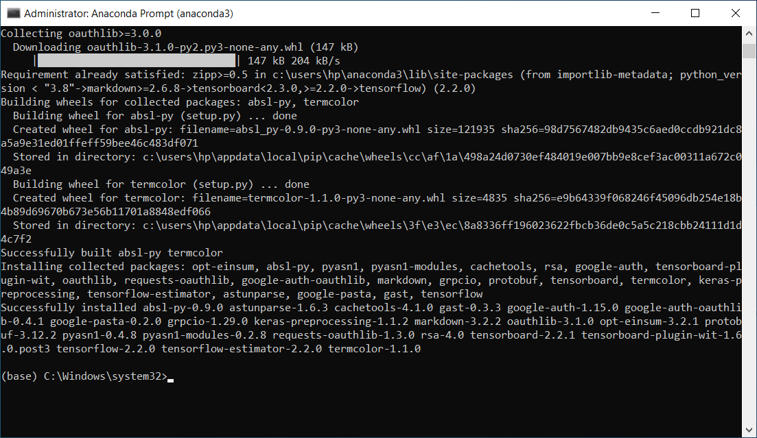
pip install keras
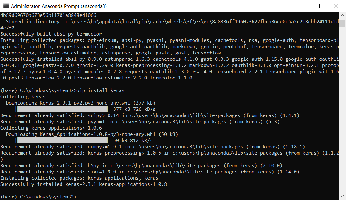
So, we have installed Keras library too. Now that we are done with the installation, the next step is to update all these libraries to the most updated version, and it can be done by following the given code. 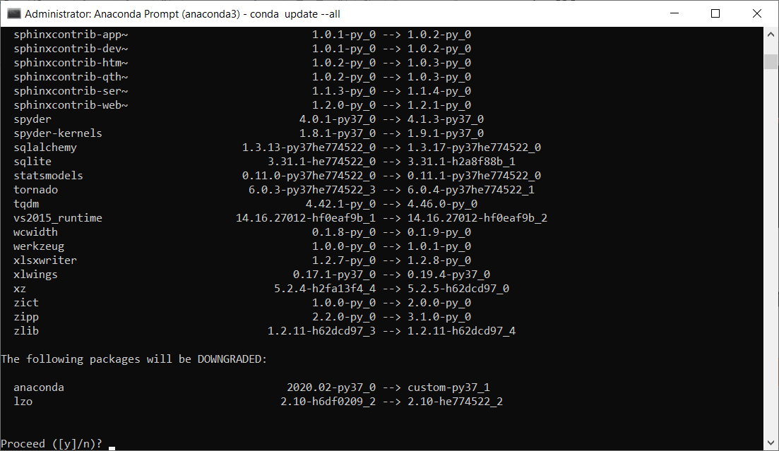
Since we are doing it for the very first time, it will ask whether to proceed or not. Confirm it with y and press enter. 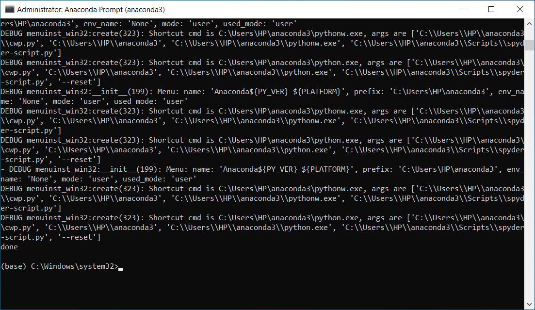
After the libraries are updated successfully, we will close the Anaconda prompt and get back to the Spyder IDE. Now we will start building our model in two parts, such that in part 1st, we will do data pre-processing, however in 2nd part, we will create the ANN model. Data pre-processing is very necessary to prepare the data correctly for building a future deep learning model. Since we are in front of a classification problem, so we have some independent variables encompassing some information about customers in a bank, and we are trying to predict the binary outcome for the dependent variable, i.e., either 1 if the customer leaves the bank or 0 if the customer stays in the bank. Part1: Data Pre-processingWe will start by importing some of the pre-defined Python libraries such as NumPy, Matplotlib, and Pandas so as to perform data-preprocessing. All these libraries perform some sort of specific tasks. NumPy NumPy is a python library that stands for Numerical Python, allows the implementation of linear, mathematical and logical operations on arrays as well as Fourier transformation and routine to manipulate the shapes. Matplotlib It is also an open-source library with the help of which charts can be plotted in the python. The sole purpose of this library is to visualize the data for which it necessitates to import its pyplot sub library. Pandas Pandas is also an open-source library that enables high-performance data manipulation as well as analyzing tools. It is mainly used to handle the data and make the analysis. An output image is given below, which shows that the libraries have been successfully imported. 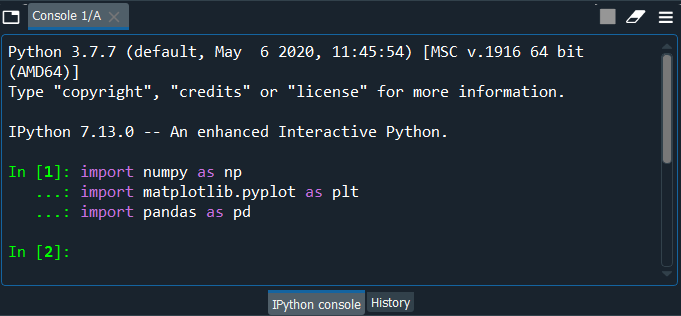
Next, we will import the data file from the current working directories with the help of Pandas. We will use read.csv() for reading the CSV file both locally as well as through the URL. From the code given above, the dataset is the name of the variable in which we are going to save the data. We have passed the name of the dataset in the read.csv(). Once the code is run, we can see that the data is uploaded successfully. By clicking on the Variable explorer and selecting the dataset, we can check the dataset, as shown in the following image. 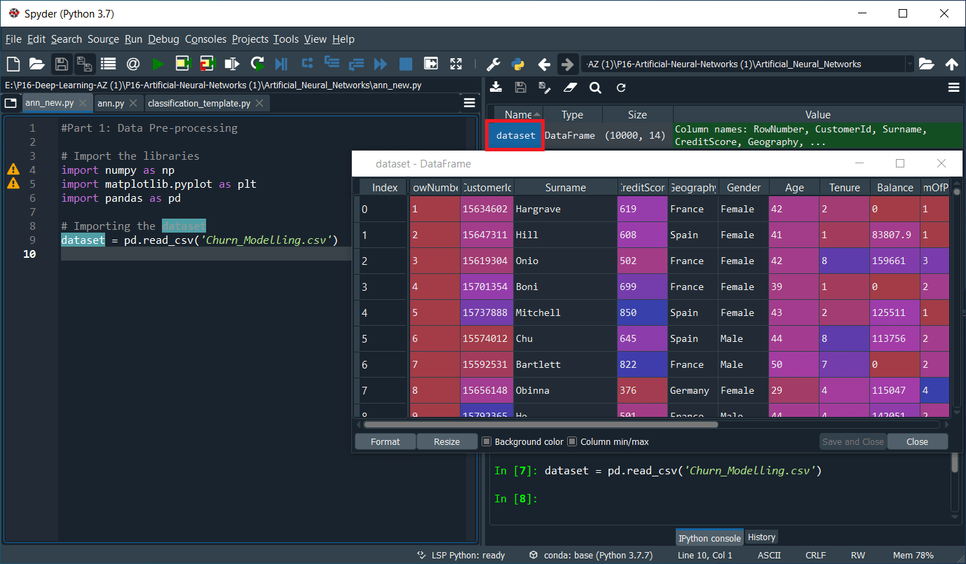
Next, we will create the matrix of feature, which is nothing but a matrix of the independent variable. Since we don't know which independent variable might has the most impact on the dependent variable, so that is what our artificial neural network will spot by looking at the correlations; it will give bigger weight to those independent variables that have the most impact in the neural network. So, we will include all the independent variables from the credit score to the last one that is the estimated salary. After running the above code, we will see that we have successfully created the matrix of feature X. Next, we will create a dependent variable vector. By clicking on y, we can have a look that y contains binary outcome, i.e., 0 or 1 for all the 10,000 customers of the bank. Output: 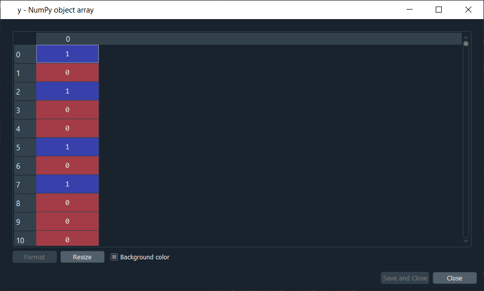
Next, we will split the dataset into the training and test set. But before that, we need to encode that matrix of the feature as it contains the categorical data. Since the dependent variable also comprises of categorical data but sidewise, it also takes a numerical value, so don't need to encode text into numbers. But then again, we have our independent variable, which has categories of strings, so we need to encode the categorical independent variables. The main reason behind encoding the categorical data before splitting is that it is must to encode the matrix of X and the dependent variable y. So, now we will encode our categorical independent variable by having a look at our matrix from console and for that we just need to press X at the console. Output: 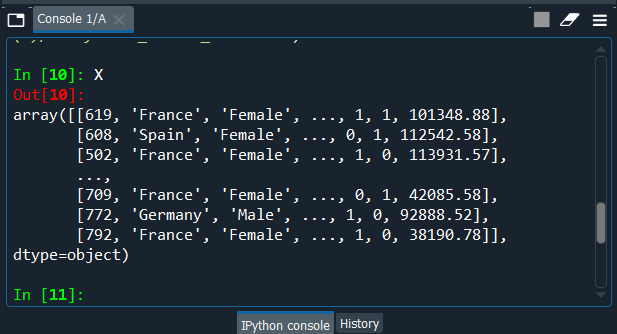
From the image given above, we can see that we have only two categorical independent variables, which is the country variable containing three countries, i.e., France, Spain, and Germany, and the other one is the gender variable, i.e., male and female. So, we have got these two variables, which we will encode in our matrix of features. So we will need to create two label encoder objects, such that we will create our first label encoder object named labelencoder_X_1 followed by applying fit_transform method to encode this variable, which will, in turn, the strings here France, Spain, and Germany into the numbers 0, 1 and 2. After executing the code, we will now have a look at the X variable, simply by pressing X in the console, as we did in the earlier step. Output: 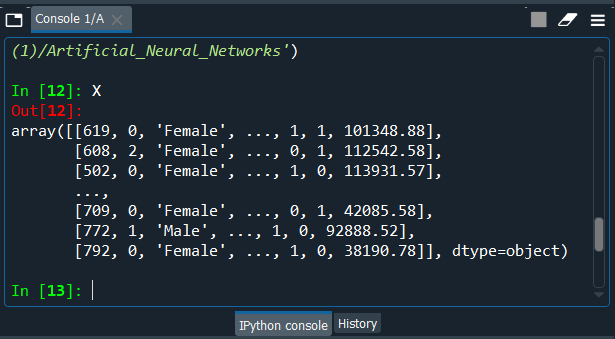
So, from the output image given above, we can see that France became 0, Germany became 1, and Spain became 2. Now in a similar manner, we will do the same for the other variable, i.e., Gender variable but with a new object. Output: 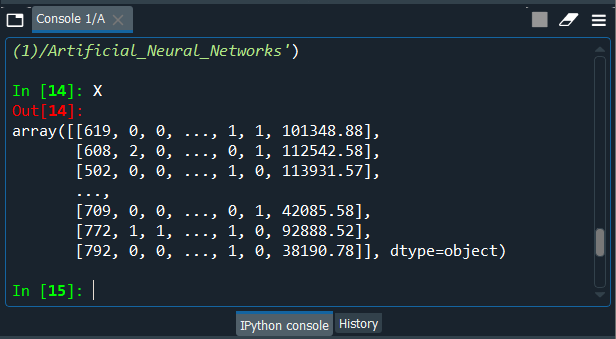
We can clearly see that females became 0 and males became 1. Since there is no relational order between the categories of our categorical variable, so for that we need to create a dummy variable for the country categorical variable as it contains three categories unlike the gender variable having only two categories, which is why we will be removing one column to avoid the dummy variable trap. It is useless to create the dummy variable for the gender variable. We will use the OneHotEncoder class to create the dummy variables. Output: 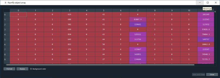
By having a look at X, we can see that all the columns are of the same type now. Also, the type is no longer an object but float64. We can see that we have twelve independent variables because we have three new dummy variables. Next, we will remove one dummy variable to avoid falling into a dummy variable trap. We will take a matrix of features X and update it by taking all the lines of this matrix and all the columns except the first one. Output: 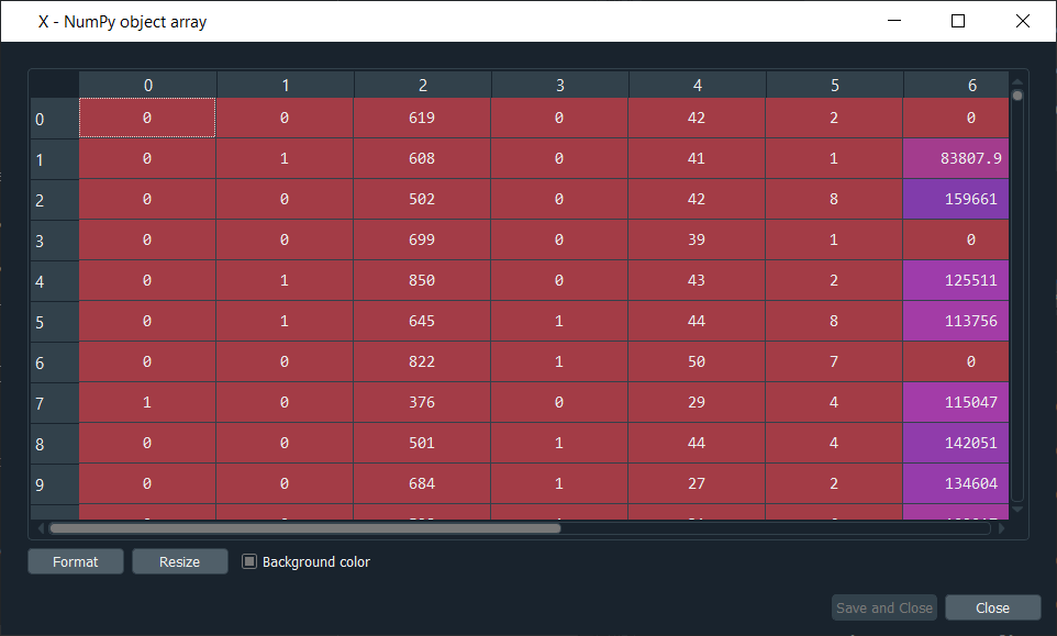
It can be seen that we are left with only two dummy variables, so no more dummy variable trap. Now we are ready to split the dataset into the training set and test set. We have taken the test size to 0.2 for training the ANN on 8,000 observations and testing its performance on 2,000 observations. By executing the code given above, we will get four different variables that can be seen under the variable explorer section. Output: 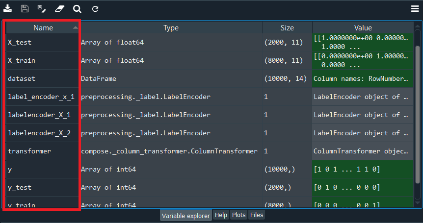
Besides parallel computations, we are going to have highly computed intensive calculations as well as we don't want one independent variable dominating the other one, so we will be applying feature scaling to ease out all the calculations. After executing the above code, we can have a quick look at X_train and X_test to check if all the independent variables are scaled properly or not. Output: X_train 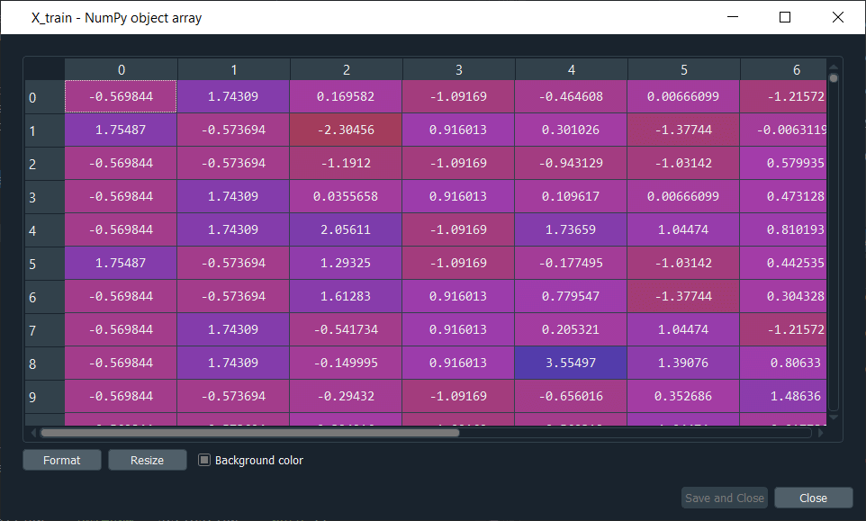
X_test 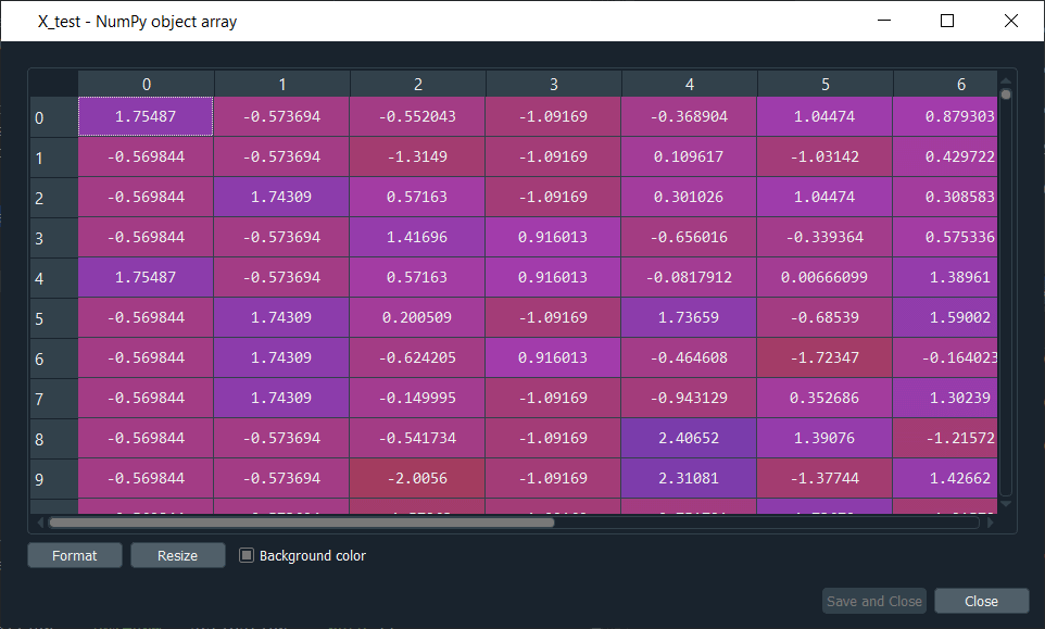
Now that our data is well pre-processed, we will start by building an artificial neural network. Part2: Building an ANNWe will start with importing the Keras libraries as well as the desired packages as it will build the Neural Network based on TensorFlow 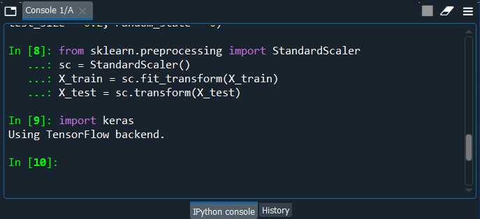
After importing the Keras library, we will now import two modules, i.e., the Sequential module, which is required to initialize our neural network, and the Dense module that is needed to build the layer of our ANN. Next, we will initialize the ANN, or simply we can say we will be defining it as a sequence of layers. The deep learning model can be initialized in two ways, either by defining the sequence of layers or defining a graph. Since we are going to make our ANN with successive layers, so we will initialize our deep learning model by defining it as a sequence of layers. It can be done by creating an object of the sequential class, which is taken from the sequential model. The object that we are going to create is nothing but the model itself, i.e., a neural network that will have a row of classifiers because we are solving a classification problem where we have to predict a class, so our neural network model is going to be a classifier. As in the next step, we will be predicting the test set result using the classifier name, so we will call our model as a classifier that is nothing but our future Artificial Neural Network that we are going to build. Since this classifier is an object of Sequential class, so we will be using it, but will not pass any argument because we will be defining the layers step by step by starting with the input layer followed by adding some hidden layers and then the output layer. After this, we will start by adding the input layer and the first hidden layer. We will take the classifier that we initialized in the previous step by creating an object of the sequential class, and we will use the add() method to add different layers in our neural network. In the add(), we will pass the layer argument, and since we are going to add two layers, i.e., the input and first hidden layer, which we will be doing with the help of Dense() function that we have mentioned above. Within the Dense() function we will pass the following arguments;
Next, we will add the second hidden layer by using the same add method followed by passing the same parameter, which is the Dense() as well as the same parameters inside it as we did in the earlier step except for the input_dim. After adding the two hidden layers, we will now add the final output layer. This is again similar to the previous step, just the fact that we will be units parameter because in the output layer we only require one node as our dependent variable is a categorical variable encompassing a binary outcome and also when we have binary outcome then, in that case, we have only one node in the output layer. So, therefore, we will put units equals to 1, and since we are in the output layer, we will be replacing the rectifier function to sigmoid activation function. As we are done with adding the layers of our ANN, we will now compile the whole artificial neural network by applying the stochastic gradient descent. We will start with our classifier object, followed by using the compile method and will pass on the following arguments in it.
Next, we will fit the ANN to the training set for which we will be using the fit method to fit our ANN to the training set. In the fit method, we will be passing the following arguments:
Output: 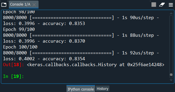
From the output image given above, you can see that our model is ready and has reached an accuracy of 84% approximately, so this how a stochastic gradient descent algorithm is performed. Part3: Making the Predictions and Evaluating the ModelSince we are done with training the ANN on the training set, now we will make the predictions on the set. Output: 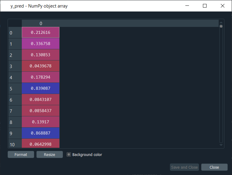
From the output image given above, we can see all the probabilities that the 2,000 customers of the test set will leave the bank. For example, if we have a look at first probability, i.e., 21% means that this first customer of the test set, indexed by zero, has a 20% chance to leave the bank. Since the predicted method returns the probability of the customers leave the bank and in order to use this confusion matrix, we don't need these probabilities, but we do need the predicted results in the form of True or False. So, we need to transform these probabilities into the predicted result. We will choose a threshold value to decide when the predicted result is one, and when it is zero. So, we predict 1 over the threshold and 0 below the threshold as well as the natural threshold that we will take is 0.5, i.e., 50%. If the y_pred is larger, then it will return True else False. Now, if we have a look at y_pred, we will see that it has updated the results in the form of "False" or "True". Output: 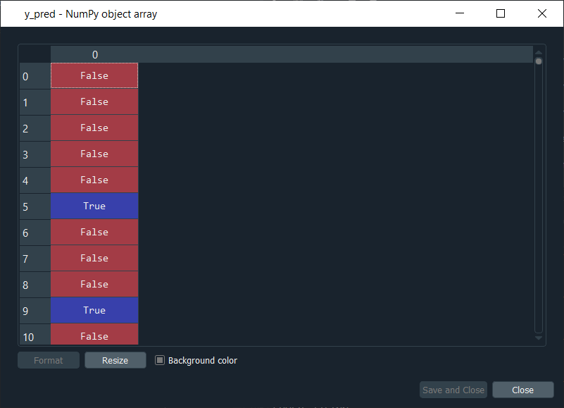
So, the first five customers of the test set don't leave the bank according to the model, whereas the sixth customer in the test set leaves the bank. Next, we will execute the following code to get the confusion matrix. Output: 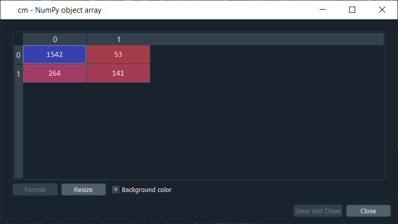
From the output given above, we can see that out of 2000 new observations; we get 1542+141= 1683 correct predictions 264+53= 317 incorrect predictions. So, now we will compute the accuracy on the console, which is the number of correct predictions divided by the total number of predictions. 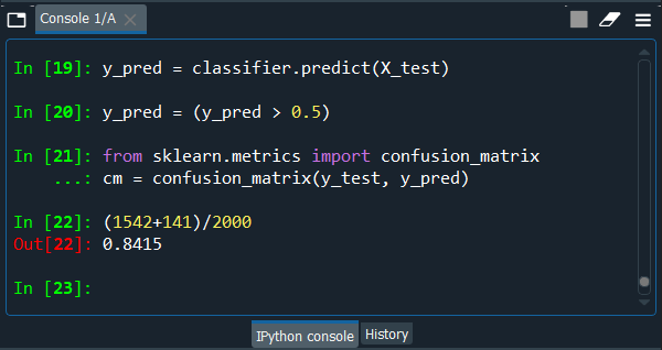
So, we can see that we got an accuracy of 84% on new observations on which we didn't train our ANN, even that get a good amount of accuracy. Since this is the same accuracy that we obtained in the training set but obtained here on the test set too. So, eventually, we can validate our model, and now the bank can use it to make a ranking of their customers, ranked by their probability to leave the bank, from the customer that has the highest probability to leave the bank, down to the customer that has the lowest probability to leave the bank.
Next TopicConvolutional Neural Network
|
 For Videos Join Our Youtube Channel: Join Now
Feedback
- Send your Feedback to [email protected]
Help Others, Please Share


Javatpoint Services
JavaTpoint offers too many high quality services. Mail us on [email protected], to get more information about given services.
- Website Designing
- Website Development
- Java Development
- PHP Development
- WordPress
- Graphic Designing
- Logo
- Digital Marketing
- On Page and Off Page SEO
- PPC
- Content Development
- Corporate Training
- Classroom and Online Training
- Data Entry
Training For College Campus
JavaTpoint offers college campus training on Core Java, Advance Java, .Net, Android, Hadoop, PHP, Web Technology and Python. Please mail your requirement at [email protected]
Duration: 1 week to 2 week


