| |

Mega Case StudyIn this mega case study, we are going to make a hybrid deep learning model. As the name suggests, this challenge is about combining two deep learning models, i.e., the Artificial Neural Network and the Self-Organizing Map. So, we will start with the credit card applications dataset to identify the frauds. The idea is to make an advanced deep learning model where we can predict the probability that each customer cheated, and to do this; we will go from unsupervised to supervised deep learning. The challenge consists of two parts, i.e., in the first part, we will make unsupervised deep learning branch of our hybrid deep learning model, and then in the second part, we will make the supervised deep learning branch that will result in the hybrid deep learning model composed of both unsupervised and supervised deep learning. Here we are again using the Credit_Card_Applications dataset that we have just seen in the self-organizing map, which contains all the credit card applications from the different customers of a bank and so we will use the self-organizing map exactly as we did in the previous topic to identify the fraud. But then there is a challenge to use the results of this self-organizing map to then combine our unsupervised deep learning model to a new supervised deep learning model that will take as input the results given by our SOM. The challenge is to obtain a ranking of the predicted probabilities that each customer cheated. We will get very small probabilities because the SOM identified only a few frauds, but that doesn't matter. The main goal is to get this ranking of the probabilities. Building a Hybrid Deep Learning ModelWe will start with Part1 that includes making an unsupervised deep learning branch of the hybrid deep learning model, i.e., the self-organizing map, which we will use to identify the frauds exactly as we did earlier. Part1: Identifying the frauds with self-organizing mapsSo, we will run the following code to get our self-organizing map that will contain the outlying neurons. Output: 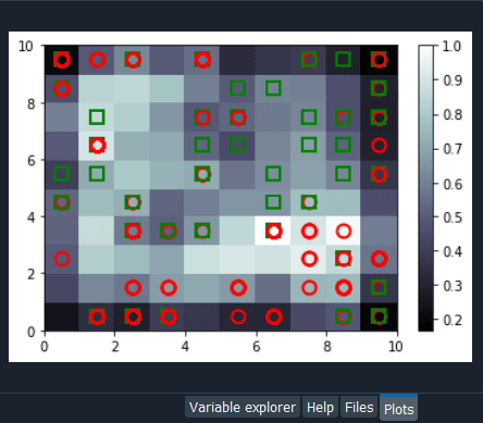
From the above image, we can see that we got an outline neuron because it is characterized by a large MID, i.e., the Mean Interneuron Distance and besides that, it contains both the categories of customers; customers that got their application approved and the customers that didn't get their application approved. So, we got the frauds for the two types of scenarios and selecting the outlying neuron is arbitrary because it depends on the threshold we want to get to select these neurons, i.e., either we want to take the whitest neurons, or we can decrease the threshold a little bit. Therefore, we will take the whitest one, and all the rest of the neurons are the regular neurons or common neurons that follow the general rules as well as they look like non-potential frauds. After now, we got the coordinates of the two neurons, as shown in the above image, i.e., the first one has coordinates (7,2), and the second one has coordinates (8,3). So, we are ready to find the frauds list, the potential frauds, which we will do by executing the following code. After executing the above code, we will go to the variable explorer and then we will click on the fraud variable where we will see that we get 17 frauds. Output: 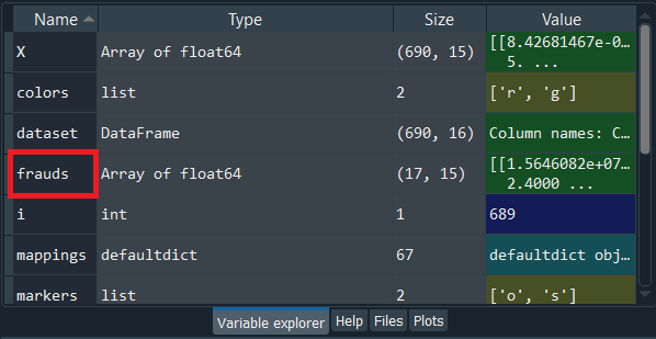
Frauds: 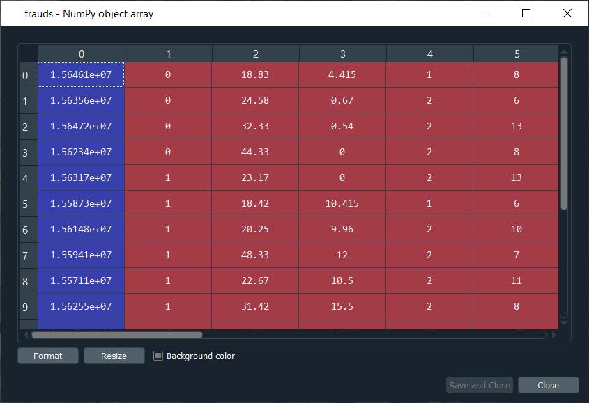
Next, we will use the list of frauds to go from unsupervised deep learning to supervised deep learning because, at the time of switching, we need a dependent variable, and with the unsupervised deep learning, we didn't consider any dependent variable for the reason that they were trained on the features without using any dependent variable. But when doing supervised learning, we need a dependent variable because we need the model to understand some correlations between the features and a result/outcome, which is in the dependent variable. Part2: Going from Unsupervised to Supervised Deep LearningIn the second part, we will first create the matrix of features, which is the first input that we will need to train our supervised learning model, and then we will create the dependent variable. To create the matrix of features, we can do the same way as we did in the previous part to extract the matrix from the dataset and for that, we will replace X with customers because this matrix of features contains the information of all the customers of the bank, such that each line corresponds to one customer with all its different information. So, we are calling it as customers, and then we will call the dependent variable as is_fraud, which is equal to 1; if yes, there is a fraud and is_fraud equals 0; if no, there is no fraud. We are taking all the columns except the last one, which is the class, whether the application was approved or not, and we included the customer ID to keep track of customers. But since we only need the matrix of features containing some information, which can potentially help predict the probability of fraud, the customer ID will not help us predict the probability of fraud. Therefore, we will not include that column, but then the last column of the database might be the relevant information that will help us identify some correlations between the customer's information and its probability to cheat. So, we never knew we would include this independent variable. To create the matrix of feature, we need all the variables from index 1, so we don't include the first one of index 0 up to the last one. Therefore, customers will be all the columns of our dataset of indexes going from 1 up to the last column and here with -1; we don't include the last column, so we will remove it. Here we include all the columns except the first one, and then, of course, we take all the lines because we want to take all the customers followed by .values to create NumPy array. By executing the above line of code, we get our feature matrix, which is shown below. Output: 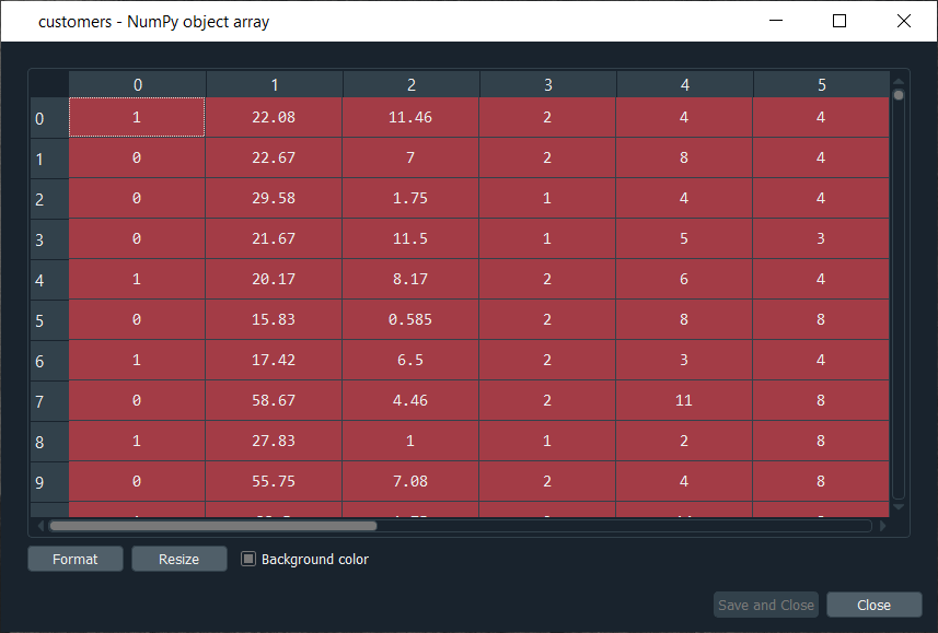
From the above image, we can see that it contains 690 customers and all their features, i.e., all the different information they need to fill out for the credit card application. Next, we will create the dependent variable, which is the trickiest part here. Since the dependent variable will contain the outcomes, whether it was a fraud or not, it will be a fraud with a binary outcome, which will get the value of 0 if there is no fraud and 1, in case there is a fraud. So, we will initialize a vector of 690 zeros, which is basically like we are pretending that at the beginning, all the customers didn't cheat and then we will extract customer IDs for which we will put a 1 in our vector of zeros. We will replace a 0 by 1 for the index corresponding to the customer ID. Let's start with initializing the vector, and as we said are going to call it as is_fraud that will be our dependent variable. Then we will initialize this vector by using a NumPy function, and for that, we will first call its shortcut np to get this function, i.e., zeros, which will create the vector of 0's of any number of elements. Since we want 690 elements, so to generalize it more, we will pass len(dataset) inside the function because it refers to the number of observations in the dataset, which is 690 in our case. After executing the above line of code, we can see that we have our vector initialized with 690 zeros in the image given below. Output: 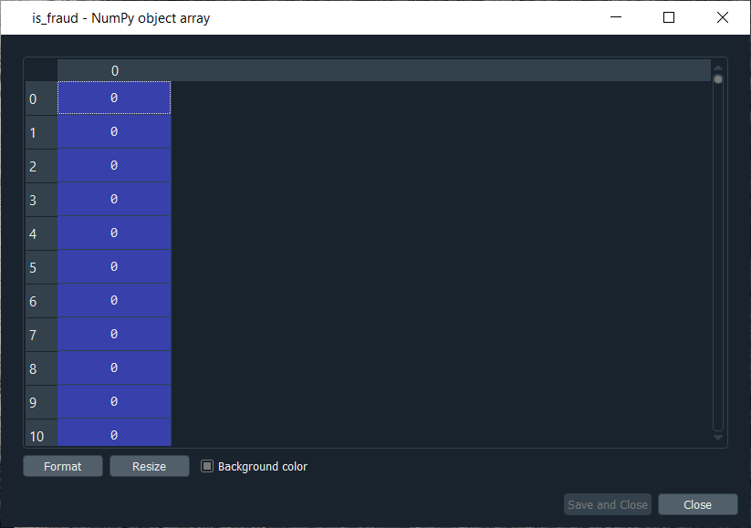
The next challenge is to put ones for all the customer ID's that potentially cheated. So, we will loop over all the customers, such that for each customer, we will check if the customer ID of the customer belongs to the list of frauds, and if that's the case, we will replace the zero by one. Therefore, we will make a for loop, then we need a variable that we call i, and then we need a range, which must be the range of the indexes of the customers, so we will write in range. Since the default start is zero, so we need to specify the stop, which is again the len(dataset), i.e., 690 followed by adding: at last. As we just said, for each customer, we need to check if its customer ID is inside the list of frauds, so we will do that by making an if condition. We will start by, if the customer ID of this customer, so we need to extract the customer ID of the customer, which is contained in the dataset.iloc[i,0], where i stands for the ith line of the dataset and as we know, each customer corresponds to a line, so the ith line corresponds to the ith customer, i.e., the customer we were dealing with just now, the loop and then 0 because as we said earlier that the first column of the contains the customer ID. So, the dataset.iloc[i,0] will get the customer ID of customer no i and then we don't need any .value because it helps in creating a NumPy array. After this, we will check if this customer ID is in the list of frauds and to that, we will add in frauds, which will look if the customer ID is inside the list of frauds. However, if that's the case, we will replace 0 by 1 for that specific customer. So, for this customer, the value in is_fraud will get a one instead of a zero, and the value of is_fraud with this customer is given by is_fraud[i] = 1, which is the value of is_fraud customer corresponding to that customer because this customer has index i. After executing the above code, we will see that our dependent variable is now a vector of 690 elements, and when we open it, we get our dependent variable with the ones for the indexes of the customers that are in the list of frauds, as shown in the below image. Since we have 17 elements in our list of frauds, so we will see that we 17 ones, which you can check by scrolling down. Output: 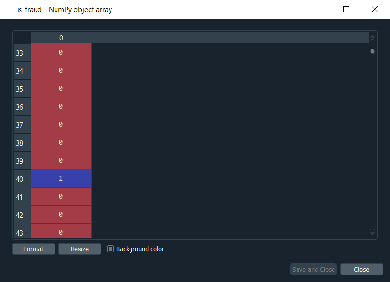
Now that we have everything to train our Artificial Neural Network, we will run the following code in the same manner as we did earlier. Basically, we are just performing the feature scaling part in all the ANN architecture, followed by the training with the fit method and then the predictions, the predicted probabilities. After running the above section, we can see from the image given below that our customers are well scaled, so we can move on to the further part. Output: 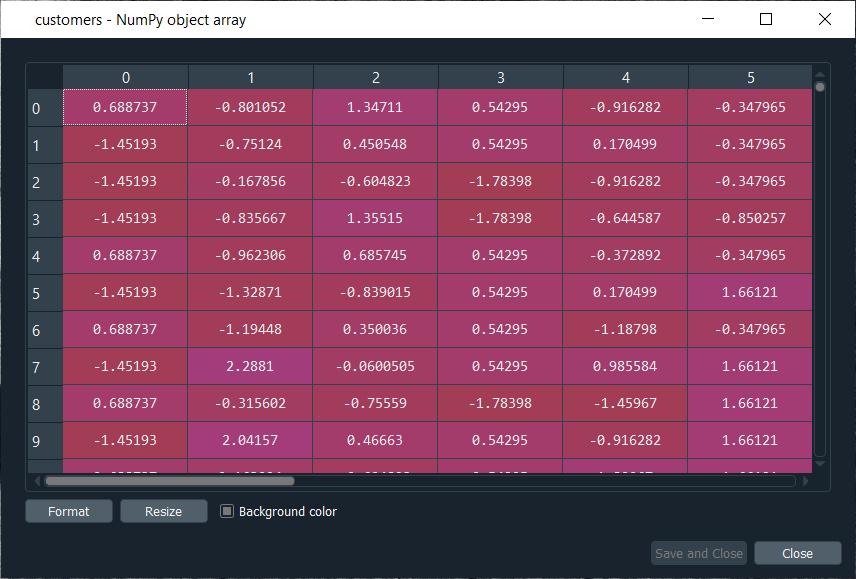
Next, we will build the Artificial Neural Network architecture and fit the ANN to our training set. There is one important thing to be noted that we are working with a very simple dataset that contains 690 observations, which is very small for our deep learning model, but the idea is not to do with big data here or work on some very complex dataset instead the idea is to learn how to combine two deep learning models. We have simplified our code as we don't need to add the complexity of the second hidden layer, so we have skipped that part, and then in the input layer, we have taken 2 neurons instead of 6 followed by changing the input dimensions as they correspond to the number of features that we have in our matrix of features. Since we have 15 features in our matrix of features, we have put input_dim equals 15 instead of 11. Also, we need to change the input, output, batch_size as well as the epochs. The input is our matrix of features, which is no longer called X_train, but now customers. Then we need to change the output, which is no longer called y_train, but now is_fraud. In order to make it simple, we have taken batch_size equals 1 and epochs equals to 2 because the dataset is so simple that it will only take 1 or 2 epochs for our Artificial Neural Network to understand the correlations. The weights will only need to be updated in 1 or 2 shots, which is why we have taken 2 epochs. You don't need to train a deep learning model for 100 epochs if you have few observations and few features. Now that we are ready with our Artificial Neural Network, we will train it to our matrix of features, customers, and our dependent variable is a fraud. After running the above code, we can see from the output image given below that we have improved accuracy, i.e., 97.54% and the loss has reduced pretty well from 45.28% to 14.64%. Output: 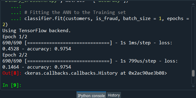
After training the Artificial Neural Network, we will move on to the next part in which we will predict the probabilities of frauds. We will put these predicted probabilities y_pred and of course, we will use our classifier followed by using the predict method not on the X_test as we did in ANN, but on the customers, because we want to predict for each customer the probability that this customer cheated or the probability that there is a fraud in its application. It will get us to the predicted probability, simply by executing the above line. After executing the above line, we can have a look at y_pred, which is given below. Output: 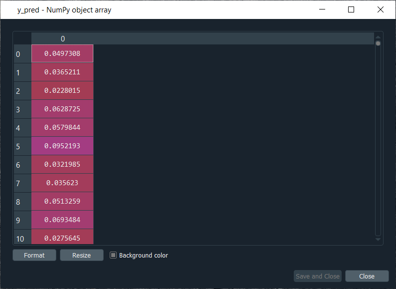
From the above image, we can see that y_pred has all the different probabilities. It has small probabilities, but that's normal because the dependent variable vector contains a few ones, i.e., only 17 out of 690 observations in total. So, this was all the probabilities, now we have to rank them and to do that, we have two options; either we can export the y_pred vector in Excel and rank the probabilities directly because in that case, we aren't required to follow it further or in order to learn some more python tricks to understand how it sorts an array in python, then we have to follow the below-given steps. But before sorting the probabilities, it will be better to include the customer IDs in the y_pred vector because, as of now, we only have the predicted probabilities. It will be great if we could create an array with two columns, where the first column will contain the customer IDs. The second column will contain the predicted probabilities so that we can clearly identify the customer who has each of the predicted probability for each customer. Let's start with adding the second column to y_pred, which will actually be in the first position, so we will again take our y_pred vector, and since we want to add our first column containing the customer IDs to the y_pred, thus we will use the same concatenate trick as we used in the earlier step. But we will make few changes; we will first get rid of the mapping, and then we will add the first column that we want to have in the 2-Dimensional array, which is, of course, the customer IDs, i.e., dataset.iloc[:, 0:1].values followed by adding the y_pred, and lastly, we will add the axis=1 because we want to make a horizontal concatenation, which is why we have taken 1 instead of 0. Now when we execute the above line, we will see in the below image that it gives us a 2D array containing two columns, i.e., the first column of the customer IDs and the second column of the predicted probabilities. Output: 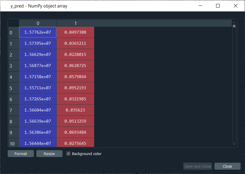
From the above image, we can see that y_pred is now a 2-Dimensional array having two columns as we expected. It has all the customer IDs in the first column and the predicted probabilities in the second column as well as we have the right association between the customer IDs and the predicted probabilities. Next, we will sort the customers by their predicted probabilities of cheating with the help of the NumPy sort function, which will sort all the columns simultaneously, but we will not do this way because we want to keep track of the customer IDs for the predicted probabilities. So, we will use a trick which will only sort our second column in no time. We will take y_pred again because we want to modify it, followed by taking y_pred[y_pred[:, 1] as it specifies what column we want to sort, which is the second column that contains the predicted probabilities. Lastly, we will use a NumPy array method, i.e., argsort(), to sort our NumPy array by the column of index 1, which is exactly what we want. Output: 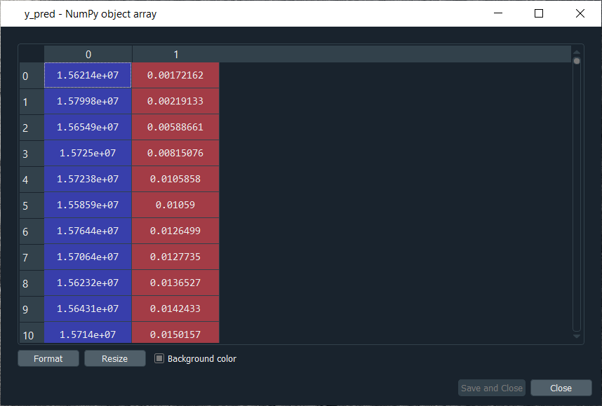
Therefore, we can see from the above image that all the probabilities are sorted from the lowest to the highest one. Hence, we got the ranking, which is much better now as the fraud department can take this ranking and investigate the fraud starting with the highest predicted probability of the fraud.
Next TopicRestricted Boltzmann Machine
|
 For Videos Join Our Youtube Channel: Join Now
Feedback
- Send your Feedback to [email protected]
Help Others, Please Share


Javatpoint Services
JavaTpoint offers too many high quality services. Mail us on [email protected], to get more information about given services.
- Website Designing
- Website Development
- Java Development
- PHP Development
- WordPress
- Graphic Designing
- Logo
- Digital Marketing
- On Page and Off Page SEO
- PPC
- Content Development
- Corporate Training
- Classroom and Online Training
- Data Entry
Training For College Campus
JavaTpoint offers college campus training on Core Java, Advance Java, .Net, Android, Hadoop, PHP, Web Technology and Python. Please mail your requirement at [email protected]
Duration: 1 week to 2 week


