| |

MATLAB PolynomialMATLAB performs, polynomials as row vectors, including coefficients ordered by descending powers. For example, the equation P(x) = x4 + 7x3 - 5x + 9 can be represented as - p = [1 7 0 -5 9]; Polynomial FunctionspolyfitGiven two vector x and y, the command a=polyfit (x, y, n) fits a polynomial of order n through the data points (xi,yi) and returns (n+1) coefficients of the power of x in the row vector a. The coefficients are arranged in the decreasing order of the power of x, i.e.,a=[a n a n-1…a 1 a 0 ]. polyvalGiven a data vector x and the coefficients of a polynomial in a row vector a the command y=polyval(a, x) evaluates the polynomials at the data points xi and generates the values yi such that yi=a(1) xn i+a(2) xi (n-1)+…+a(n)x+a(n+1). Hence, the length of the vector a is n+1, and, consequently, the order of the evaluated polynomial is n. Thus if a is 5 elements long, the polynomial to be evaluated is automatically ascertained to be of the fourth-order. Both polyfit and polyval use an optimal argument if you need error estimates. Example: Straight-line (linear) fitThe following data is collected from an experiment aimed at measuring the spring constant of a given spring. Different masses m are hung from the spring, and the corresponding deflections δ of the spring from its unstretched configuration are measured. From physics, we have that F=kδ and here F=mg. Thus, we can find k from the relationship k=mg/δ. Here, we are going to find k by plotting the experimental data, fitting the best straight line (we know that the relationship between δ and F is linear) through the data, and then measuring the slope of the best-fit line.
Fitting a straight line through the data means we want to find the polynomial coefficients a1 and a0(a first-order polynomial) such that a1 xi+a0gives the "best" estimate of yi. In steps, we need to the following: Step1: Find the coefficients ak' s: a=polyfit(x, y, 1) Step2: Evaluate y at finer (more closely spaced) xj' s using the fitted polynomial: y_fitted=polyval(a, x_fine) Step3: Plot and see. Plot the given input as points and fitted data as a line: plot(x, y, 'o',x_fine, y_fitted); Following script file shows all the steps contained in making a straight-line fit through the given data for the spring experiment and finding the spring constant. And plots the following graph: 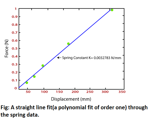
Least squares curve fittingThe procedure of least square curve fit can simply be implemented in MATLAB, because the technique results in a set of linear equations that need to be solved. Most of the curve fits are polynomial curve fits or exponential curve fits (including power laws, e.g., y=axb). Two most commonly used functions are:
1.ln (y)=ln (a) +bx or y =a0+a1 x,where y =ln(y), a1=b,and a0=ln?(a). 2. ln(y)=ln(c) +d ln (x) or y = a0+a1 x, where y = ln (y), a1=d,and a0=ln?(c). Now we can use polyfit in both methods with just first-order polynomials to determine the unknown constants. The steps involved are the following: Step1: Develop new input: Develop new input vectors y and x, as allocate, by taking the log of the original input. For example, to fit the curve of the type y=aebx, create ybar=log(y) and leave x and to fit a curve of the type y=cxd, create ybar=log(y) and xbar=log(x). Step2: Do a linear fit: Use polyfit to found the coefficients a0 and a1for a linear curve fit. Step3: Plot the curve: From the curve fit coefficients, calculates the values of the original constants (e.g., a, b). Recomputed the values of y at the given x's according to the relationship obtained and plot the curve along with the original data. The following are the table shows the time versus pressure variation readings from a vacuum pump. We will fit a curve, P(t)=P0 e-t/τ, through the data, and determine the unknown constants P0 and τ.
By taking the log of both sides of the relationships, we have 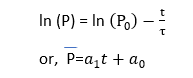
where P=ln(P), a1= Example: Create a script file And plots the following graph: 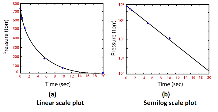
Next TopicMATLAB Interpolation
|
 -and a0=ln?(P0 ). Thus, we can easily computed P0 and τ once we have a1 and a0.
 For Videos Join Our Youtube Channel: Join Now
Feedback
- Send your Feedback to [email protected]
Help Others, Please Share


Javatpoint Services
JavaTpoint offers too many high quality services. Mail us on [email protected], to get more information about given services.
- Website Designing
- Website Development
- Java Development
- PHP Development
- WordPress
- Graphic Designing
- Logo
- Digital Marketing
- On Page and Off Page SEO
- PPC
- Content Development
- Corporate Training
- Classroom and Online Training
- Data Entry
Training For College Campus
JavaTpoint offers college campus training on Core Java, Advance Java, .Net, Android, Hadoop, PHP, Web Technology and Python. Please mail your requirement at [email protected]
Duration: 1 week to 2 week


